Classifying Jake Arrieta’s Pitch Types

Major League Baseball currently has high definition cameras capturing everything from the release point of the ball being thrown to the amount of horizontal movement on the pitch and even the spin rate of the ball. Rather than having a human manually track and record the type of pitch for each pitch thrown, an algorithm does this automatically. The goal of this analysis is to use MLB’s classifications to run a neural network of my own that will match that of Major League Baseball.

The training dataset being used is from all of Jake Arrieta’s pitches thrown in the 2016 regualar season and the model is validated against 98 pitches that Arrieta threw in Game 2 of the 2016 World Series.

# Load in the required packages
library(nnet)
library(caret)
library(pitchRx)
library(dplyr)
library(plyr)
library(RSQLite)
library(devtools)

The following script was used to scrape data from the 2016 season and filtered for Jake Arrieta’s pitches. A similar script was ran for only data on 10/26/16, the date of Game 2 from the 2016 World Series.

db2016 <- src_sqlite("MLB2016_All.sqlite3", create = FALSE)
scrape(start = "2016-04-01", end = "2016-10-01", connect = db2016$con)

locations <- select(tbl(db2016, "pitch"), 
                    pitch_type, start_speed, end_speed, num, gameday_link,
                    pfx_x, pfx_z, vx0, vy0, vz0, ax, ay, az, break_y, 
                    break_angle, break_length, spin_dir, spin_rate)
names <- select(tbl(db2016, "atbat"), pitcher_name, batter_name, 
                num, gameday_link, stand)
que <- inner_join(locations, filter(names, pitcher_name == "Jake Arrieta"),
                  by = c("num", "gameday_link"))

pitchfx <- collect(que, n=Inf)
pitchfx <- as.data.frame(pitchfx)
arrieta <- subset(pitchfx, select = -c(pitcher_name, batter_name, stand, num, gameday_link))

# import function for plotting nnet
source_url('https://gist.githubusercontent.com/fawda123/7471137/raw/466c1474d0a505ff044412703516c34f1a4684a5/nnet_plot_update.r')

# Read in 2016 season data and Game 2 of the World Series
arrieta <- read.csv('~/arrieta.csv')
validation <- read.csv('~/world_series.csv')

# Split the regular season data into a new training and testing set.
intrain <- createDataPartition(arrieta$pitch_type, p=0.7, list=FALSE)
myTrain <- arrieta[intrain,]
myTest <- arrieta[-intrain,]
head(myTrain)

Example of the dataset. A glossary of the PITCHf/x fields can be seen here.

  pitch_type start_speed end_speed pfx_x pfx_z    vx0      vy0     vz0      ax     ay      az
       SL        91.2      85.3  4.30  4.92  6.892 -133.311  -7.881   7.829 25.485 -23.139
       SI        94.6      87.4 -9.14  5.68  9.580 -138.194  -7.213 -17.751 29.649 -21.066
       FF        92.6      84.7 -7.68  9.66 12.007 -135.195  -4.506 -14.149 30.639 -14.305
       SI        92.5      84.2 -8.14  7.79 11.627 -134.928  -7.360 -14.827 32.771 -17.919
       SI        94.0      85.1 -9.72  8.95 12.134 -137.136  -5.906 -18.203 35.086 -15.348
       FF        94.1      87.3 -6.69  9.64 10.836 -136.968 -12.245 -12.816 27.952 -13.644
  break_y break_angle break_length spin_dir spin_rate
  23.9       -20.1          5.8  139.091  1301.037
  23.8        35.0          5.7  237.962  2198.319
  23.8        36.8          4.2  218.372  2445.865
  23.7        31.6          5.2  226.126  2211.533
  23.7        42.0          4.9  227.250  2622.399
  23.8        33.7          4.1  214.668  2386.429

Neural Network from nnet Package

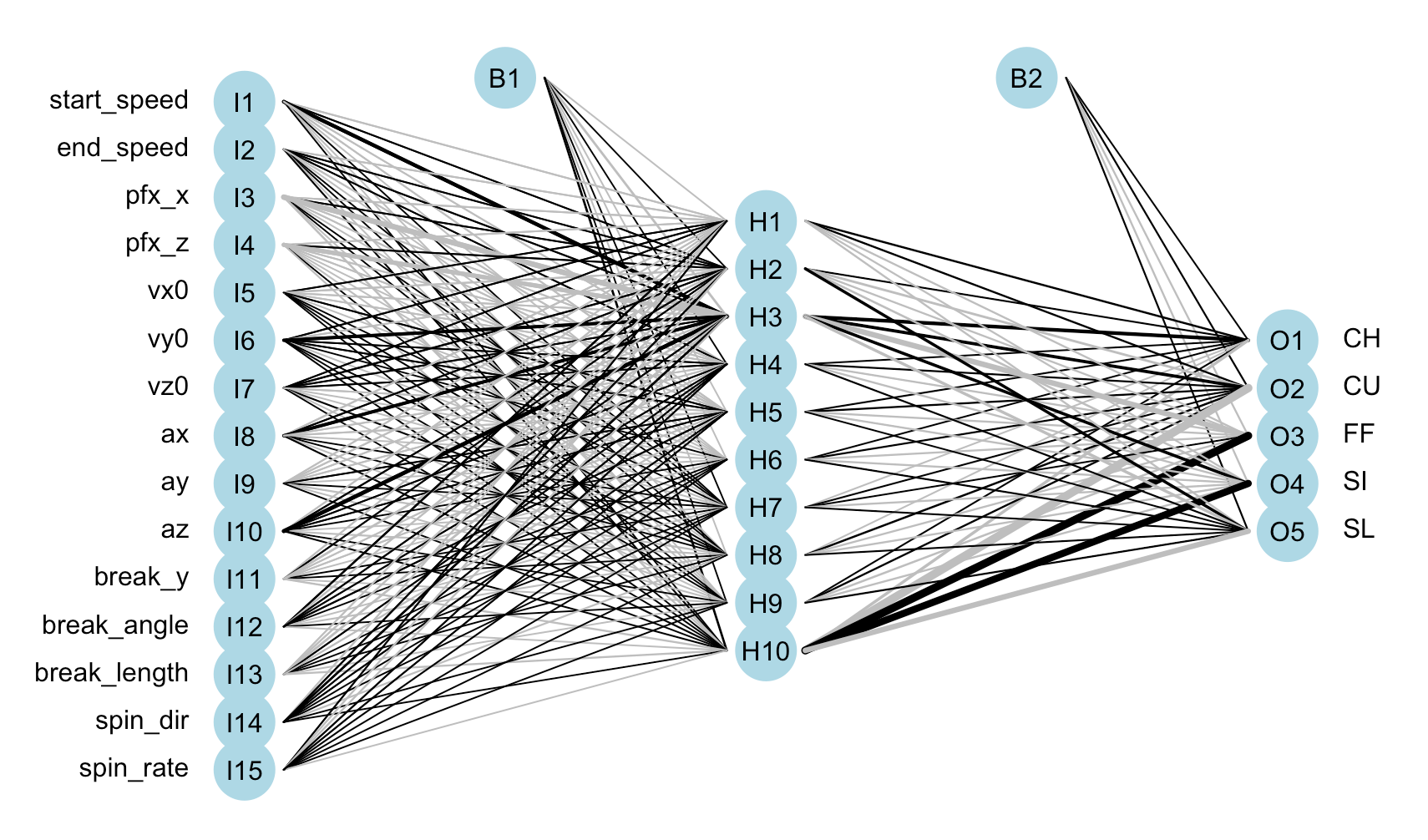
This is a simple feed-forward neural network with a single hidden layer. More complicated methods were tested by using Keras and Theano, but those methods proved to be not necessary for this type of classification.

set.seed(353)
nn_mod1 <- nnet(pitch_type ~ ., data = myTrain, 
           size = 10, rang = 0.1, decay = 5e-04, 
           maxit = 1000)

test.pred <- predict(nn_mod1, newdata = myTest, type = "class")
table(test.pred, myTest$pitch_type)

test.pred  CH  CU  FF  SI  SL
       CH  41   0   0   0   0
       CU   2 113   0   1   2
       FF   1   0 189   2   1
       SI   0   0   2 411   0
       SL   0   1   1   0 165

# plot each model
plot.nnet(nn_mod1)

This image shows the layout of the neural network with 15 input nodes (features), 10 hidden nodes and 5 output nodes (pitch types).

plot of image1

# structure (15 inputs, 10 hidden layers, 5 outputs)
nn_mod1$n

# summary of model
summary(nn_mod1)

This summary gives an example of the weight and bias values between each node. The table can be read as: the bias value to the first hidden node is 0.0, the weight from the first input node to the first hidden node is -0.44, the weight from the second input node to the first hidden ndoe is -0.38, etc.

plot of image2

Validate Model Against New Dataset

# Validation on new data from 2016 World Series game 2
val.pred <- predict(nn_mod1, newdata = validation, type = "class")

# Misclassified Pitch number 13
table(val.pred, validation$pitch_type)
confusionMatrix(val.pred, validation$pitch_type)

The confusion matrix shows that the model misclassified one pitch out of the 98 thrown by Arrieta in Game 2 of the World Series. The thirteenth pitch he threw was a sinker and my model classified the pitch as a four-seam fastball. We can take a look at the actual video footage to see why the model may have been wrong. As it turns out, this particular pitch was not thrown well by Arrieta.

          Reference
Prediction CH CU FF SI SL
        CH  1  0  0  0  0
        CU  0 15  0  0  0
        FF  0  0 49  1  0
        SI  0  0  0 11  0
        SL  0  0  0  0 21

Analysis

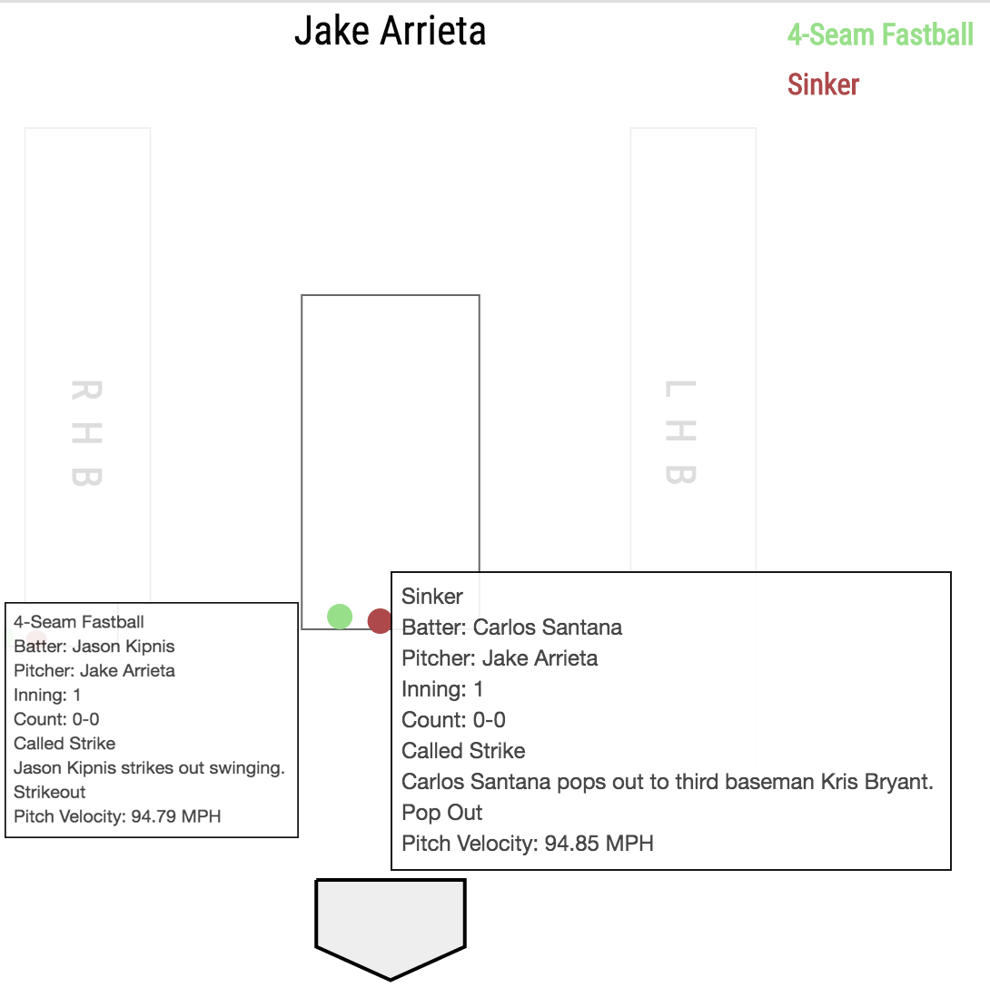
First, let’s take a look at a four-seam fastball and a sinker thrown by Arrieta to show how similar these pitches look and how difficult it would be for a human to classify. The below image shows one of each pitch thrown in the first inning from Game 2, both in nearly the same location and almost identical pitch velocities.

plot of chunk image3 Image from Baseball Savant

Play the videos of each pitch and see for yourself if you would have been able to identify the difference.

Pitch 1: Sinker

Video from MLB.com

Pitch 4: Four-Seam Fastball

Video from MLB.com

Misclassified Pitch

Pitch 13 in the video below was marked by MLB as being a sinker and misclassified in my model as a four-seam fastball. Arrieta missed his spot by throwing the ball far outside of the strike zone and one might assume that he did not throw this pitch well. It appears that there may be a very small, downward cut on the pitch, thus identifying the ball as a sinker, but it is very difficult to detect with the naked eye. The table below shows how subtle the differences can be by looking at the mean of various factors grouped by pitch type. Arrieta gets more spin on his sinker than compared to his four-seam fastball, but only a computer can pick up that information.

detach(package:plyr)
mean.group <- validation %>% 
  group_by(pitch_type) %>% 
  summarise (mean_break_angle = mean(break_angle), 
  mean_break_length = mean(break_length),
  mean_spin_rate = mean(spin_rate), 
  mean_spin_dir = mean(spin_dir))
as.data.frame(mean.group)

  pitch_type mean_break_angle mean_break_length mean_spin_rate mean_spin_dir
       CH         26.60000          5.800000       1957.302     228.09300
       CU        -16.50667         13.326667       1976.298      50.75767
       FF         26.34082          4.057143       2162.419     209.88673
       SI         31.75000          5.125000       2132.878     226.50800
       SL        -18.04286          7.695238       1120.785     107.67705

Pitch 13: Sinker

Video from MLB.com

Conclusion

Overall, it is clear that you do not need a very complicated model for predicting pitch types. This model showed to have a 98.9% accuracy and even then, there are often times pitches that cannot be categorized as one type of pitch or another for various reasons.